Explore Fatou sets & fractals

Julia package for Fatou sets. Install using Pkg.add("Fatou") in Julia. See https://github.com/chakravala/Fatou.jl for source code. This package provides: fatou, juliafill, mandelbrot, newton, basin, plot, and orbit; along with various internal functionality using Reduce and Julia expressions to help compute Fatou.FilledSet efficiently. Full documentation is included. The fatou function can be applied to a Fatou.Define object to produce a Fatou.FilledSet, which can then be passed as an argument to the plot function of PyPlot. Creation of Fatou.Define objects is done via passing a function expression (in variables z, c) and optional keyword arguments to juliafill, mandelbrot, and newton.

Background

This package enables users of Julia lang to easily generate, explore, and share fractals of Julia, Mandelbrot, and Newton type. The name Fatou comes from the mathematician after whom the Fatou sets are named. Note that the Julia language is not named after the mathematician Julia after whom the Julia sets are named. This is a mere coincidence.

Definition (Julia set): For any holomorphic function on a complex plane, the boundary of the set of points whose result diverges when function is iteratively evaluated at points.

Definition (Fatou set): The Julia set’s complement is the set of fixed limit points from holomorphic recursion.

Definition (Mandelbrot set): The set of points on a complex parameter space for which the holomorphic recursion does not go to infinity from a common starting point z0.

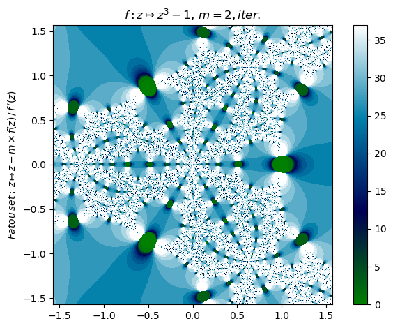
Definition (Newton fractal): The Julia/Fatou set obtained from the recursion of the Newton method z↦z−m⋅f(z)/f′(z) applied to a holomorphic function.

The package has essentially two different plotting modes controlled by the iter boolean keyword, which toggles whether to color the image by iteration count or whether to use a default (or custom) limit-value coloring function.

The number of Julia threads available is detected at the startup and is reported it back. When a specified Fatou set is computed, multi-threading is used to compute the pixels. Since each pixel is independent of any other pixel, it doesn’t matter in what order or on how many threads it is computed, the more you use the faster it is. The environment variable JULIA_NUM_THREADS is used to enable multi-threading for more than 1 thread.

Please share your favorite fractals as Fatou snippet in the discussion thread!

Example details & plotting

Fatou.Define provides the following optional keyword arguments:

Q::Expr 	= :(abs2(z)),           # escape criterion, (z, c) -> Q
C::Expr 	= :((angle(z)/(2π))*n^p)# coloring, (z, n=iter., p=exp.) -> C
∂    = π/2, # Array{Float64,1}      # Bounds, [x(a),x(b),y(a),y(b)]
n::Integer  = 176,                  # vertical grid points
N::Integer  = 35,                   # max. iterations
ϵ::Number   = 4,                    # basin ϵ-Limit criterion
iter::Bool  = false,                # toggle iteration mode
p::Number   = 0,                    # iteration color exponent
newt::Bool  = false,                # toggle Newton mode
m::Number   = 0,                    # Newton multiplicity factor
mandel::Bool= false,                # toggle Mandelbrot mode
seed::Number= 0.0+0.0im,            # Mandelbrot seed value
x0          = nothing,              # orbit starting point
orbit::Int  = 0,                    # orbit cobweb depth
depth::Int  = 1,                    # depth of function composition
cmap::String= ""                    # imshow color map

A Fatou set is a collection of complex valued orbits of an iterated function. To help illustrate this, an additional feature is a plot function designed to visualize real-valued-orbits. Fatou can be initialized with using Fatou, PyPlot or ImageInTerminal.

When using ImageInTerminal, the display of a Fatou.FilledSet will be plotted automatically in the terminal. The orbit method also has optional UnicodePlots compatibility. Additional plotting support can be added via Pull-Request by adding another Requires script to the __init__() function definition.

Basic Usage (filled-in Julia set)

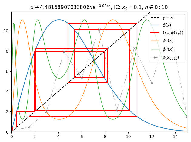
Another feature is a plot function designed to visualize real-valued-orbits. The following is a cobweb orbit plot of a function:

juliafill(:(z^2-0.67),∂=[-1.25,1.5],x0=1.25,orbit=17,depth=3,n=147) |> orbit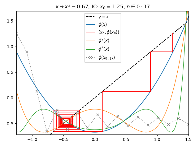

With fatou and plot it is simple to display a filled in Julia set:

c = -0.06 + 0.67im
nf = juliafill(:(z^2+$c),∂=[-1.5,1.5,-1,1],N=80,n=1501,cmap="gnuplot",iter=true)
plot(fatou(nf), bare=true)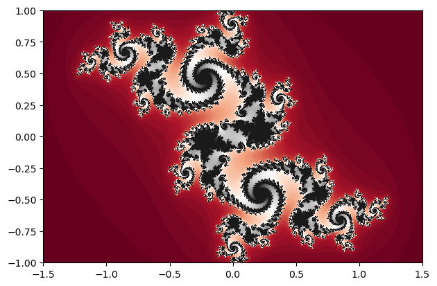

It is also possible to switch to mandelbrot mode:

mandelbrot(:(z^2+c),n=800,N=20,∂=[-1.91,0.51,-1.21,1.21],cmap="gist_earth") |> fatou |> plot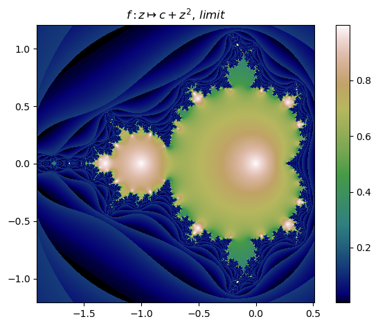

Generalized Newton basin fractals

Another type are the Julia sets of the generalized Newton's method,

\[ z \mapsto z - m \frac{f(z)}{f'(z)}.) \]

Consider the polynomial map f = :(z^3-1) with variable m = 1. To get a Julia function that applies the Newton method to this formula use η = Fatou.newton_raphson(f,m). Repeated function composition converges towards cube-root of 1. For example,

julia>  ξ = Fatou.funk(η); ζ = 2.1; [ξ(ζ,0), [Fatou.recomp(η,ζ,k) for k ∈ 2:4]...]
4-element Array{Float64,1}:
 1.47559
 1.13681
 1.01581
 1.00024

This package comes with a plot function designed to visualize real-valued-orbits. The following is a cobweb orbit plot of the function with the Newton method applied to it using

newton(:(z^3-1),∂=[0.4,2.5],x0=2.1,orbit=4,depth=2,n=42) |> orbit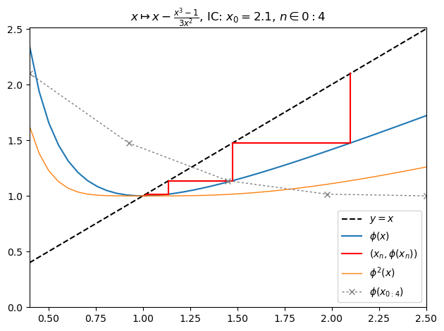

The set of points that are within an ϵ neighborhood of the roots ri of the function f is

\[ D_0(\epsilon) = \left\{ z\in\mathbb{C}: \left|\,z - r_i\,\right|<\epsilon,\,\forall r_i(\,f(r_i)=0 )\right\}) \]

Fatou also provides basin to display the the Newton / Fatou basins using set notation in LaTeX in IJulia.

map(display,[basin(newton(:(z^3-1)),i) for i ∈ 1:3])

\[ D_1(\epsilon) = \left\{z\in\mathbb{C}:\left|\,z - \frac{z^{3} - 1}{3 z^{2}} - r_i\,\right|<\epsilon,\,\forall r_i(\,f(r_i)=0 )\right\}) \] \[ D_2(\epsilon) = \left\{z\in\mathbb{C}:\left|\,z - \frac{\left(z - \frac{z^{3} - 1}{3 z^{2}}\right)^{3} - 1}{3 \left(z - \frac{z^{3} - 1}{3 z^{2}}\right)^{2}} - \frac{z^{3} - 1}{3 z^{2}} - r_i\,\right|<\epsilon,\,\forall r_i(\,f(r_i)=0 )\right\}) \] \[ D_3(\epsilon) = \left\{z\in\mathbb{C}:\left|\,z - \frac{\left(z - \frac{\left(z - \frac{z^{3} - 1}{3 z^{2}}\right)^{3} - 1}{3 \left(z - \frac{z^{3} - 1}{3 z^{2}}\right)^{2}} - \frac{z^{3} - 1}{3 z^{2}}\right)^{3} - 1}{3 \left(z - \frac{\left(z - \frac{z^{3} - 1}{3 z^{2}}\right)^{3} - 1}{3 \left(z - \frac{z^{3} - 1}{3 z^{2}}\right)^{2}} - \frac{z^{3} - 1}{3 z^{2}}\right)^{2}} - \frac{\left(z - \frac{z^{3} - 1}{3 z^{2}}\right)^{3} - 1}{3 \left(z - \frac{z^{3} - 1}{3 z^{2}}\right)^{2}} - \frac{z^{3} - 1}{3 z^{2}} - r_i\,\right|<\epsilon,\,\forall r_i(\,f(r_i)=0 )\right\}) \]

Now compute the Newton fractal Julia set for a function with annotated plot of root convergents (1):

newton(:(z^3-1),ϵ=0.001,n=800,cmap="brg") |> fatou |> plot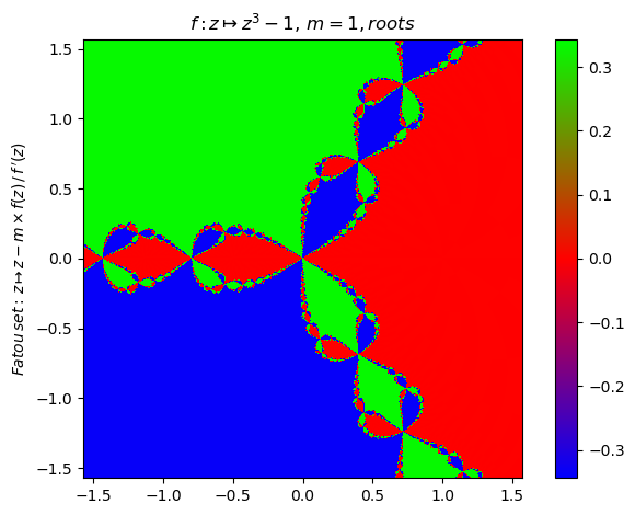

Compute the Newton fractal Julia set for a function with annotated plot of iteration count:

nf = newton(:(z^3-1),n=800,ϵ=0.1,N=25,iter=true,cmap="jet")
nf |> fatou |> plot
basin(nf,3)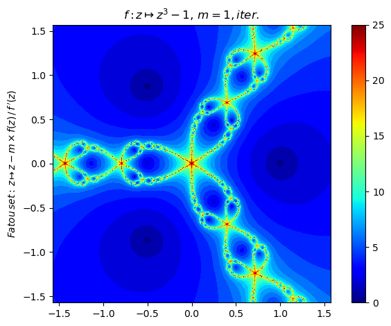

\[ D_3(\epsilon) = \left\{z\in\mathbb{C}:\left|\,z - \frac{\left(z - \frac{\left(z - \frac{z^{3} - 1}{3 z^{2}}\right)^{3} - 1}{3 \left(z - \frac{z^{3} - 1}{3 z^{2}}\right)^{2}} - \frac{z^{3} - 1}{3 z^{2}}\right)^{3} - 1}{3 \left(z - \frac{\left(z - \frac{z^{3} - 1}{3 z^{2}}\right)^{3} - 1}{3 \left(z - \frac{z^{3} - 1}{3 z^{2}}\right)^{2}} - \frac{z^{3} - 1}{3 z^{2}}\right)^{2}} - \frac{\left(z - \frac{z^{3} - 1}{3 z^{2}}\right)^{3} - 1}{3 \left(z - \frac{z^{3} - 1}{3 z^{2}}\right)^{2}} - \frac{z^{3} - 1}{3 z^{2}} - r_i\,\right|<\epsilon,\,\forall r_i(\,f(r_i)=0 )\right\}) \]

Now change the multiplicity parameter m from 1 to 2 (2). # Repeated function composition produces further singularities:

nf = newton(:(z^3-1),m=2,n=800,N=37,ϵ=0.27,iter=true,cmap="ocean",orbit=17,depth=3)
orbit(z->nf.F(z,0), [-π 2π -1],17,3,147); PyPlot.ylim(-2,7)
nf |> fatou |> plot
basin(nf,3)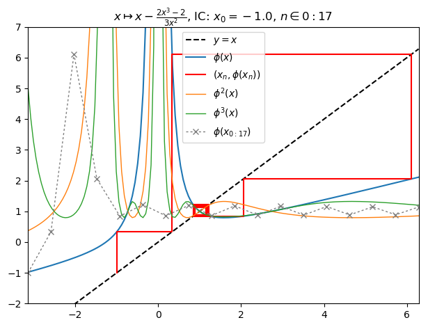

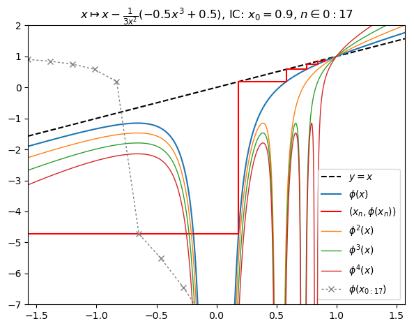
\[ D_3(\epsilon) = \left\{z\in\mathbb{C}:\left|\,z - \frac{2 \left(z - \frac{2 \left(z - \frac{2 z^{3} - 2}{3 z^{2}}\right)^{3} - 2}{3 \left(z - \frac{2 z^{3} - 2}{3 z^{2}}\right)^{2}} - \frac{2 z^{3} - 2}{3 z^{2}}\right)^{3} - 2}{3 \left(z - \frac{2 \left(z - \frac{2 z^{3} - 2}{3 z^{2}}\right)^{3} - 2}{3 \left(z - \frac{2 z^{3} - 2}{3 z^{2}}\right)^{2}} - \frac{2 z^{3} - 2}{3 z^{2}}\right)^{2}} - \frac{2 \left(z - \frac{2 z^{3} - 2}{3 z^{2}}\right)^{3} - 2}{3 \left(z - \frac{2 z^{3} - 2}{3 z^{2}}\right)^{2}} - \frac{2 z^{3} - 2}{3 z^{2}} - r_i\,\right|<\epsilon,\,\forall r_i(\,f(r_i)=0 )\right\}) \]

Set multiplicity parameter to m = -0.5 for this generalized Newton fractal (3):

nf = newton(:(z^3-1),m=-0.5,n=800,N=10,cmap="hsv",x0=0.9,orbit=17,depth=4)
nf |> fatou |> plot
orbit(nf); PyPlot.ylim(-7,2)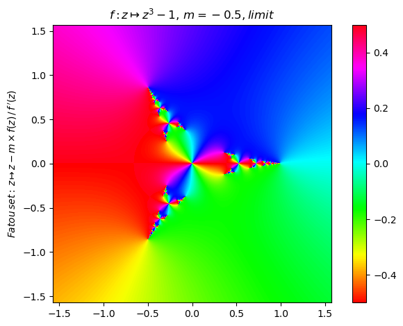

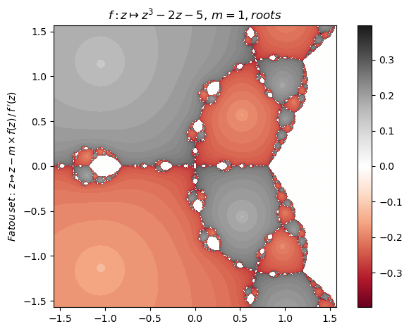
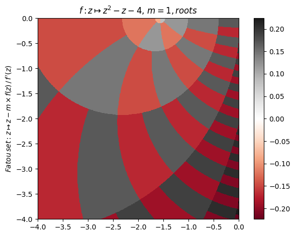
Change polynomial function (4):

nf = newton(:(z^3-2z-5),n=800,p=0.3,cmap="RdGy")
orbit(z->nf.F(z,0), [-1.5π π/2 0.2],27,2,147); PyPlot.ylim(-11,3)
nf |> fatou |> plot
basin(nf,2)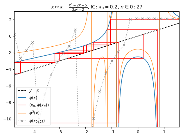

\[ D_2(\epsilon) = \left\{z\in\mathbb{C}:\left|\,z - \frac{- 2 z + \left(z - \frac{z^{3} - 2 z - 5}{3 z^{2} - 2}\right)^{3} - 5 + \frac{2 z^{3} - 4 z - 10}{3 z^{2} - 2}}{3 \left(z - \frac{z^{3} - 2 z - 5}{3 z^{2} - 2}\right)^{2} - 2} - \frac{z^{3} - 2 z - 5}{3 z^{2} - 2} - r_i\,\right|<\epsilon,\,\forall r_i(\,f(r_i)=0 )\right\}) \]

Generalized Newton fractal example (5):

newton(:(z^2-1),m=1+1im,∂=π/2.4,n=800,N=10,cmap="hsv") |> fatou |> plot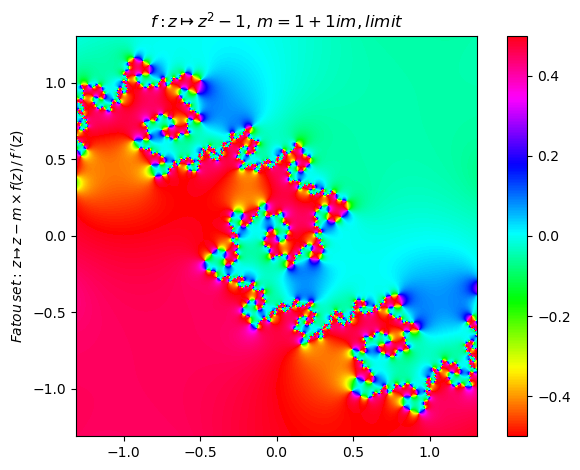

Generalized Newton fractal example (6):

newton(:(z^2-im),m=-0.5+2im,n=800,N=10,cmap="hsv") |> fatou |> plot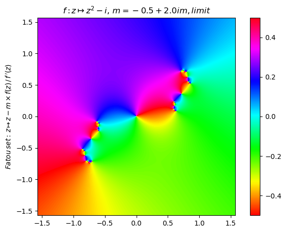

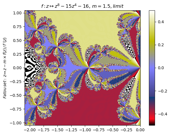
Generalized Newton fractal example (7):

nf = newton(:(z^8-15z^4-16),m=1.5,∂=[-2π/3,0,-π/3,π/3],n=1501,N=17,cmap="gist_stern",x0=-1,orbit=17,depth=3)
nf |> orbit; PyPlot.ylim(-3,7)
nf |> fatou |> plot
basin(nf,1)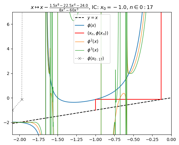

\[ D_1(\epsilon) = \left\{z\in\mathbb{C}:\left|\,z - \frac{1.5 z^{8} - 75961.5}{8 z^{7}} - r_i\,\right|<\epsilon,\,\forall r_i(\,f(r_i)=0 )\right\}) \]

Generalized Newton fractal example (8):

newton(:(z^8-15z^4-16),m=-0.5+2im,∂=[-2π/3,0,-π/3,π/3],n=500,N=10,cmap="hsv") |> fatou |> plot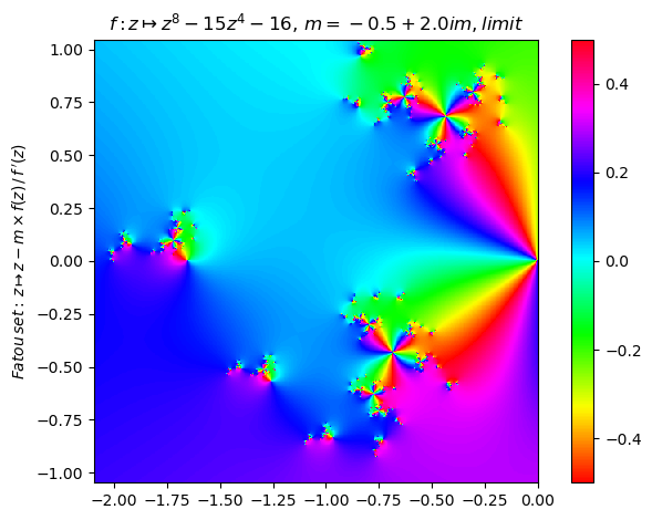

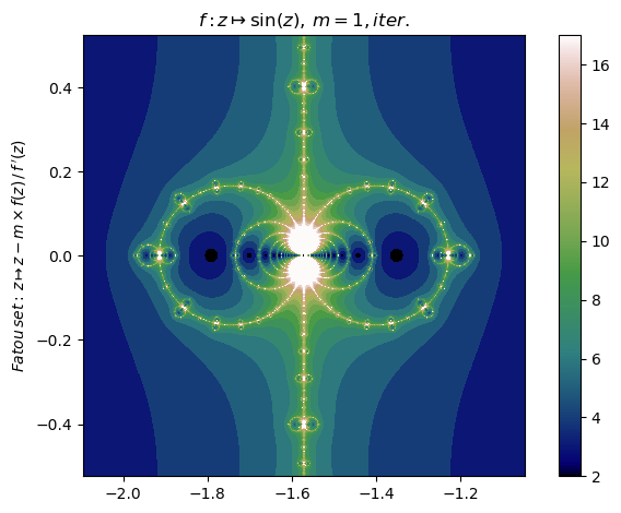
Generalized Newton fractal example (9):

nf=newton(:(sin(z)),m=1,∂=[-2π/3,-π/3,-π/6,π/6],n=800,N=17,iter=true,cmap="gist_earth",x0=-1.5,orbit=17,depth=3)
nf |> orbit; PyPlot.ylim(-30,30)
nf |> fatou |> plot
basin(nf,3)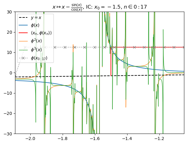

\[ D_3(\epsilon) = \left\{z\in\mathbb{C}:\left|\,z - \frac{\sin{\left (z \right )}}{\cos{\left (z \right )}} - \frac{\sin{\left (z - \frac{\sin{\left (z \right )}}{\cos{\left (z \right )}} \right )}}{\cos{\left (z - \frac{\sin{\left (z \right )}}{\cos{\left (z \right )}} \right )}} + \frac{\sin{\left (- z + \frac{\sin{\left (z \right )}}{\cos{\left (z \right )}} + \frac{\sin{\left (z - \frac{\sin{\left (z \right )}}{\cos{\left (z \right )}} \right )}}{\cos{\left (z - \frac{\sin{\left (z \right )}}{\cos{\left (z \right )}} \right )}} \right )}}{\cos{\left (- z + \frac{\sin{\left (z \right )}}{\cos{\left (z \right )}} + \frac{\sin{\left (z - \frac{\sin{\left (z \right )}}{\cos{\left (z \right )}} \right )}}{\cos{\left (z - \frac{\sin{\left (z \right )}}{\cos{\left (z \right )}} \right )}} \right )}} - r_i\,\right|<\epsilon,\,\forall r_i(\,f(r_i)=0 )\right\}) \]

Generalized Newton fractal example (10):

nf = newton(:(sin(z)-1),m=1-1im,∂=[-2π/3,-π/3,-π/6,π/6],n=800,N=33,iter=true,ϵ=0.05,cmap="cubehelix")
nf |> fatou |> plot
basin(nf,2)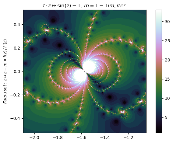

\[ D_2(\epsilon) = \left\{z\in\mathbb{C}:\left|\,z - \frac{1}{\cos{\left (z \right )}} \left(1 + i\right) \left(\sin{\left (z \right )} - 1\right) - \frac{\left(1 + i\right) \left(\sin{\left (z - \frac{1}{\cos{\left (z \right )}} \left(1 + i\right) \left(\sin{\left (z \right )} - 1\right) \right )} - 1\right)}{\cos{\left (z - \frac{1}{\cos{\left (z \right )}} \left(1 + i\right) \left(\sin{\left (z \right )} - 1\right) \right )}} - r_i\,\right|<\epsilon,\,\forall r_i(\,f(r_i)=0 )\right\}) \]

Generalized Newton fractal example (11):

nf = newton(:(z^6+z^3-1),m=(1-0.4im),∂=[-0.5,0.5,-1,0],n=800,N=33,ϵ=1e-7,
        p=0.7,cmap="YlGnBu",C="(-angle(z)/(2π))*n^e")
nf |> fatou |> plot
basin(nf,1)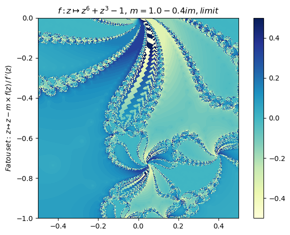

\[ D_1(\epsilon) = \left\{z\in\mathbb{C}:\left|\,z - \frac{\left(1.0 + 0.4 i\right) \left(z^{6} - z^{3} - 1\right)}{6 z^{5} - 3 z^{2}} - r_i\,\right|<\epsilon,\,\forall r_i(\,f(r_i)=0 )\right\}) \]

Generalized Newton fractal example (12):

newton(:(cos(z)-1),m=-0.5+2im,n=350,N=15,ϵ=0,cmap="hsv") |> fatou |> plot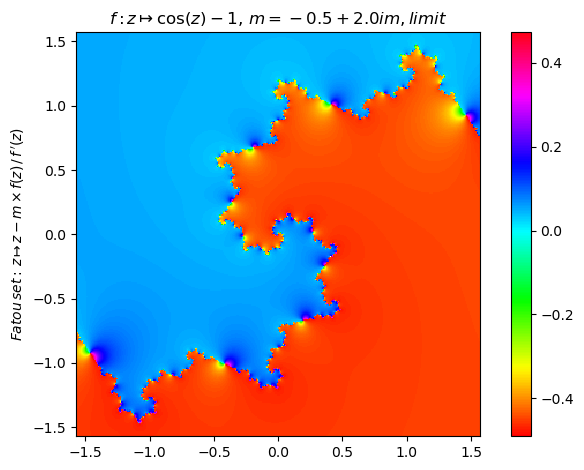

newton(:(cos(z)-1),m=0.5-2im,n=350,N=15,ϵ=0,cmap="hsv") |> fatou |> plot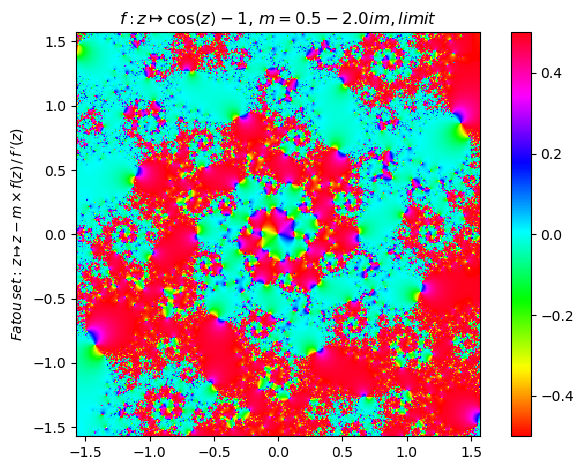

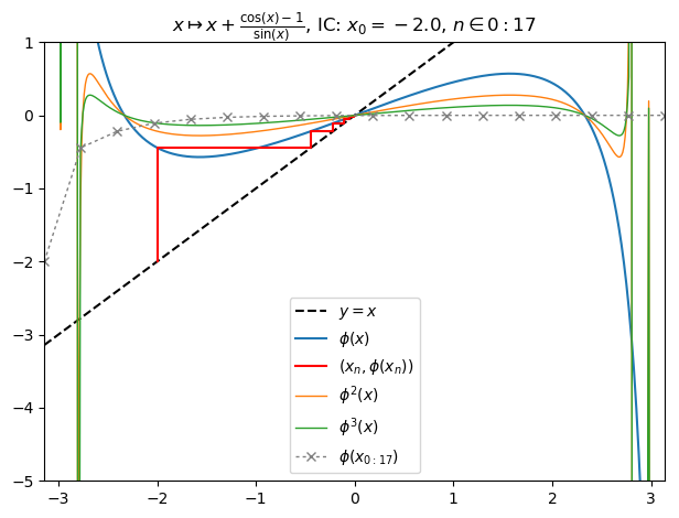
Generalized Newton fractal example (13):

nf = newton(:(cos(z)-1),m=1,∂=π,n=500,N=35,ϵ=0,cmap="YlGnBu",x0=-2,orbit=17,depth=3)
nf |> fatou |> plot
display(basin(nf,2))
orbit(nf); PyPlot.ylim(-5,1)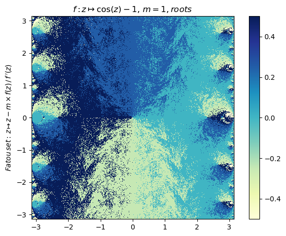

\[ D_2(\epsilon) = \left\{z\in\mathbb{C}:\left|\,z + \frac{\cos{\left (z \right )} - 1}{\sin{\left (z \right )}} + \frac{\cos{\left (z + \frac{\cos{\left (z \right )} - 1}{\sin{\left (z \right )}} \right )} - 1}{\sin{\left (z + \frac{\cos{\left (z \right )} - 1}{\sin{\left (z \right )}} \right )}} - r_i\,\right|<\epsilon,\,\forall r_i(\,f(r_i)=0 )\right\}) \]

Generalized Newton fractal example (14):

nf = newton(:(z^5-3im*z^3-(5+2im)z^2+3z+1),m=1-0.24im,∂=2.0,n=800,ϵ=0.01,iter=true,N=27,cmap="brg") 
nf |> fatou |> plot
basin(nf,1)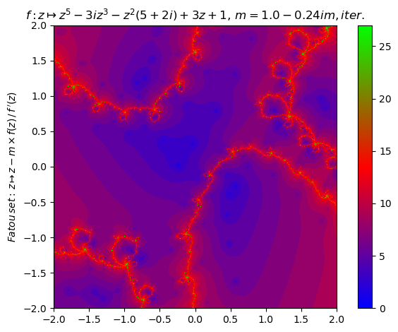

\[ D_1(\epsilon) = \left\{z\in\mathbb{C}:\left|\,z - \frac{\left(1.0 - 0.24 i\right) \left(z^{5} - 3 i z^{3} - z^{2} \left(5 + 2 i\right) + 3 z + 1\right)}{5 z^{4} - 9 i z^{2} - 2 z \left(5 + 2 i\right) + 3} - r_i\,\right|<\epsilon,\,\forall r_i(\,f(r_i)=0 )\right\}) \]

Generalized Newton fractal example (15):

nf = newton(:(log(z)),m=1+1im,∂=2π,n=500,N=27,cmap="brg")
nf |> fatou |> plot
basin(nf,2)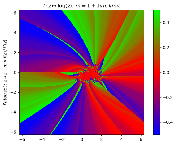

\[ D_1(\epsilon) = \left\{z\in\mathbb{C}:\left|\,- z \left(1 - i\right) \log{\left (z \right )} + z - r_i\,\right|<\epsilon,\,\forall r_i(\,f(r_i)=0 )\right\}) \]

Generalized Newton fractal example (16):

nf = newton(:(z^(4.0+3.0im)-1),m=2.1,∂=π,n=500,N=27,cmap="terrain")
nf |> fatou |> plot
basin(nf,1)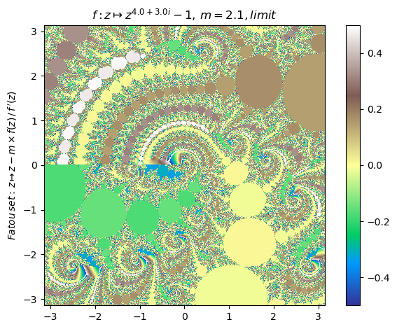

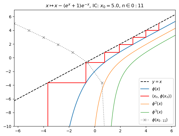
\[ D_1(\epsilon) = \left\{z\in\mathbb{C}:\left|\,- \frac{z z^{-4 - 3 i}}{4 + 3 i} \left(2.1 z^{4 + 3 i} - 2.1\right) + z - r_i\,\right|<\epsilon,\,\forall r_i(\,f(r_i)=0 )\right\}) \]

Generalized Newton fractal example (17):

nf = newton(:(e^z+1),m=1,∂=2π,n=800,iter=true,N=27,cmap="brg",x0=5,orbit=11,depth=3)
orbit(nf); PyPlot.ylim(-10,7)
nf |> fatou |> plot
basin(nf,2)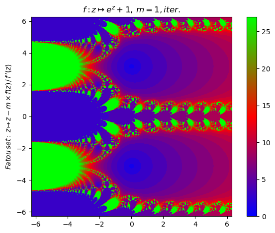

\[ D_2(\epsilon) = \left\{z\in\mathbb{C}:\left|\,z - \left(e^{z} + 1\right) e^{- z} - \left(e^{z - \left(e^{z} + 1\right) e^{- z}} + 1\right) e^{- z + \left(e^{z} + 1\right) e^{- z}} - r_i\,\right|<\epsilon,\,\forall r_i(\,f(r_i)=0 )\right\}) \]

More orbit examples

Orbit example (1):

juliafill("z*exp(1.5*(1-z^2/50))",∂=[0,15],x0=1,orbit=24) |> orbit
juliafill("z*exp(1.5*(1-z^2/50))",∂=[0,15],x0=0.1,orbit=10,depth=3) |> orbit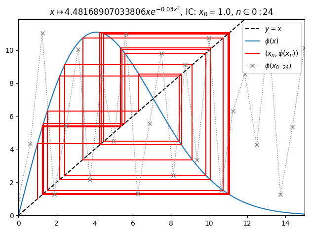

Orbit example (2):

juliafill("z*exp(1.5*(1-z/50))",∂=[0,64],x0=1,orbit=10,depth=2) |> orbit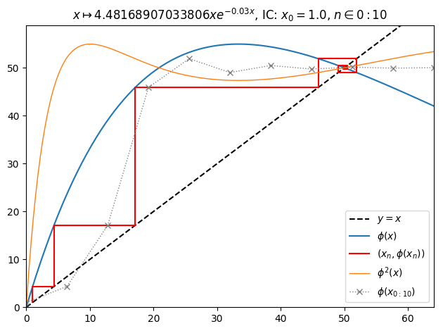

Orbit example (3):

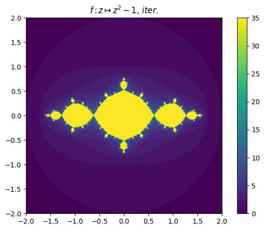
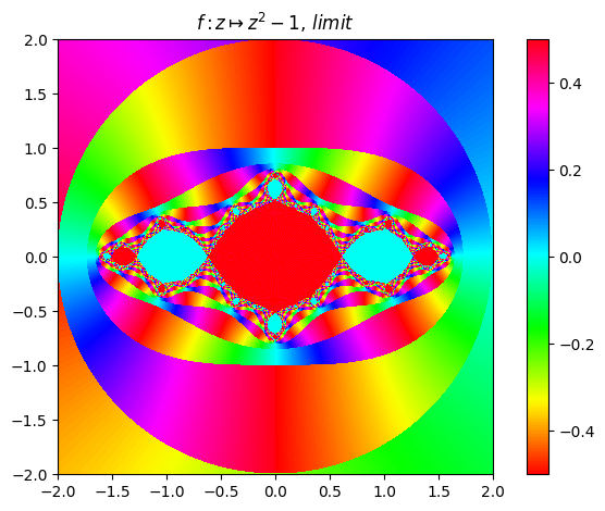
juliafill("z^2-1",∂=[-2,2],x0=0,orbit=10,depth=5) |> orbit
juliafill("z^2-1",∂=[-2,2],iter=true,n=800) |> fatou |> plot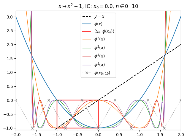

Orbit example (4):

juliafill("z^2+1.",∂=[-2,2],n=800,cmap="hsv") |> fatou |> plot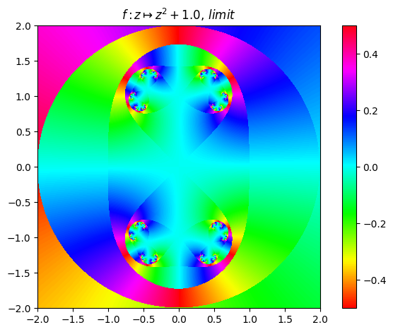

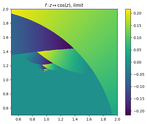
Orbit example (5):

juliafill("cos(z)",∂=[0,2],x0=1.7,orbit=17,depth=3) |> orbit
juliafill("cos(z)",∂=[0.5,2],n=500) |> fatou |> plot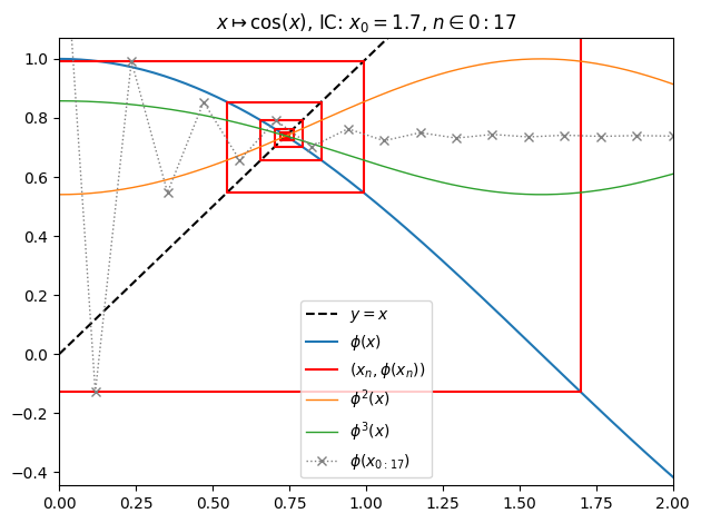

Orbit example (6):

juliafill("z^2-1",∂=[-2,2],x0=sqrt(2),orbit=10,depth=5) |> orbit
juliafill("z^2-1",∂=[-2,2],cmap="hsv",n=800) |> fatou |> plot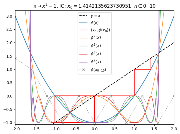

Orbit example(7):

juliafill("sin(z)",∂=[0,2],n=700) |> fatou |> plot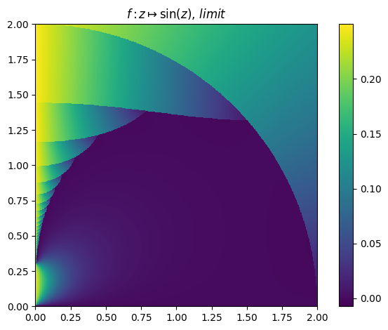

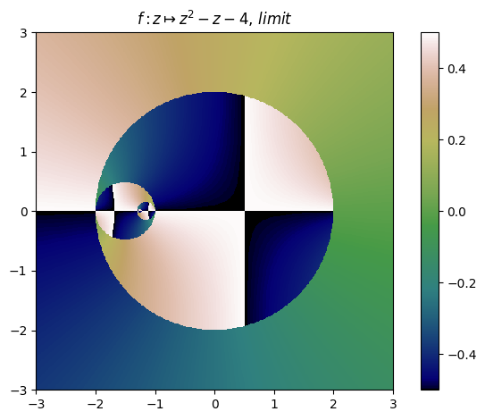
Orbit example (8):

juliafill("z^2-z-4",∂=[-4,4],x0=0.99999999+sqrt(5),orbit=37,depth=3) |> orbit
juliafill("z^2-z-4",∂=[-3,3],n=500,cmap="gist_earth") |> fatou |> plot
newton("z^2-z-4",∂=[-4,0],n=700,cmap="RdGy",p=0.5) |> fatou |> plot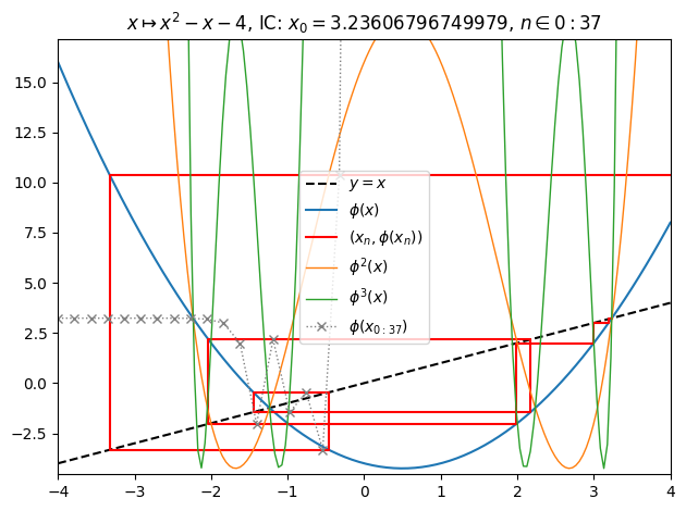

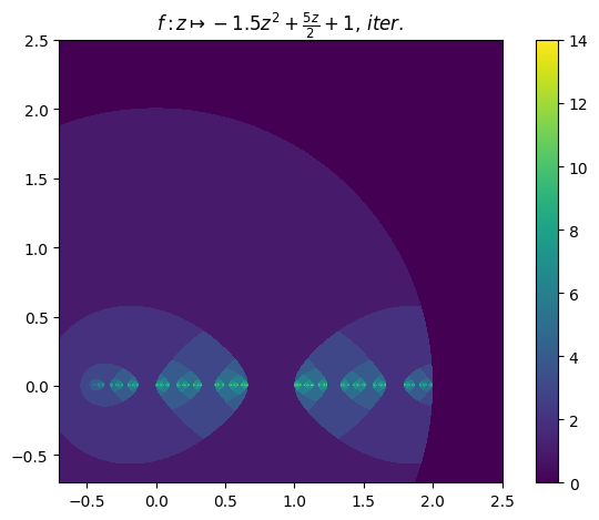
Orbit example (9):

juliafill("(-3/2)*z^2+5z/2+1",∂=[-0.7,2.5],x0=0.001,orbit=37,depth=3) |> orbit
juliafill("(-3/2)*z^2+5z/2+1",∂=[-0.7,2.5],n=800,iter=true) |> fatou |> plot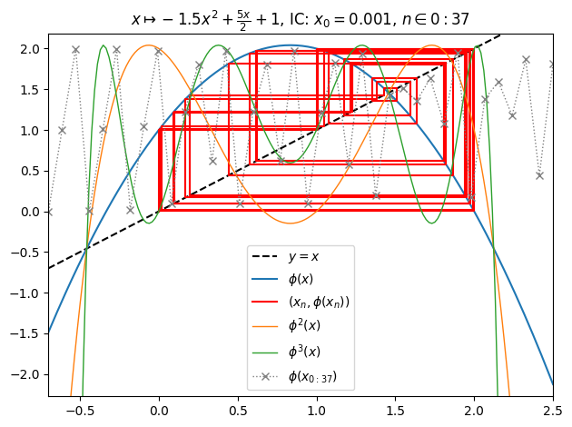

Orbit example (10):

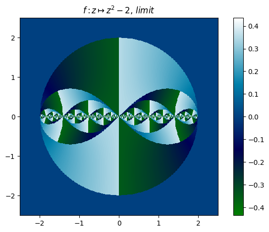
juliafill("z^2-2",∂=[-2.5,2.5],x0=0.01,orbit=100) |> orbit
juliafill("z^2-2",∂=[-2.5,2.5],n=500,p=0.1,cmap="ocean") |> fatou |> plot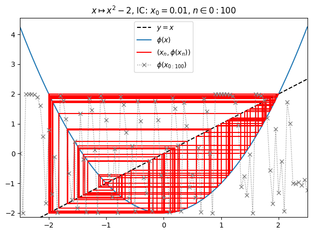

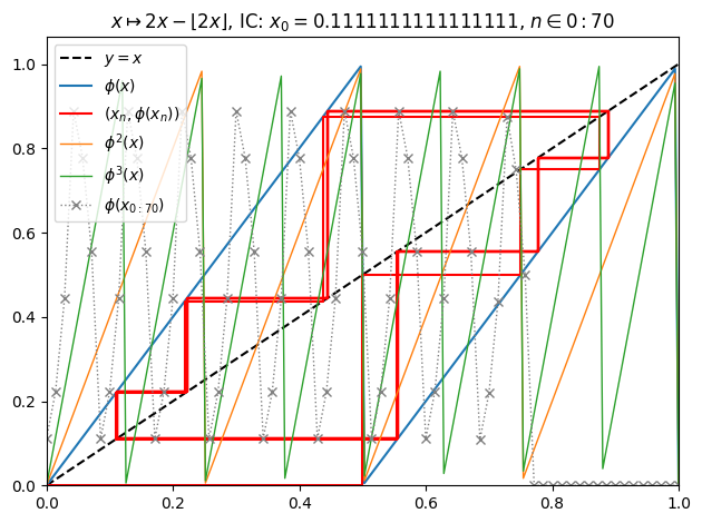
Orbit example (11):

juliafill("2z%1",∂=[0,1],x0=0.3,orbit=70,depth=3) |> orbit
juliafill("2z%1",∂=[0,1],x0=1/9,orbit=70,depth=3) |> orbit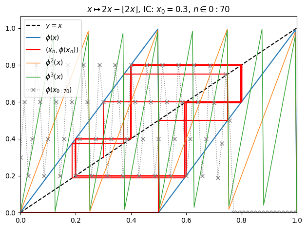

Orbit example (12):

juliafill("z^3",∂=[0,2],n=500,cmap="ocean") |> fatou |> plot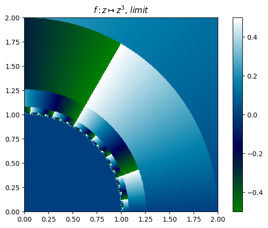

Orbit example (13):

juliafill("sqrt(z)",∂=[-3.2,6.4],cmap="ocean",n=500) |> fatou |> plot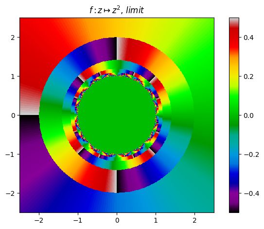

Orbit example (14):

juliafill("z^2+1",∂=[-2.5,2.5],n=500,cmap="nipy_spectral") |> fatou |> plot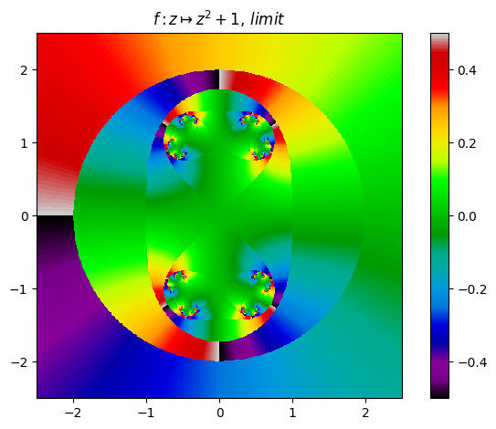

Orbit example (15):

juliafill("z^2-2",∂=[-2.5,2.5],n=500,cmap="nipy_spectral") |> fatou |> plot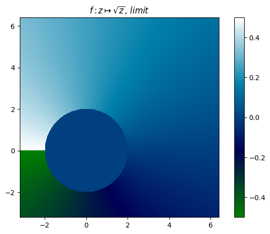

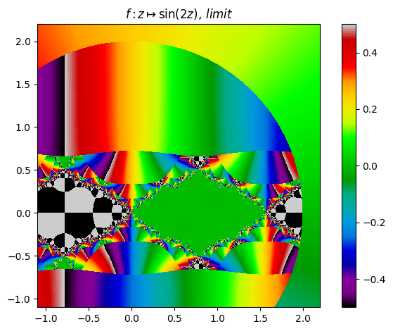
Orbit example (16):

juliafill("sin(2z)",∂=[-0.5pi,pi],x0=1.5,orbit=17,depth=4) |> orbit
juliafill("sin(2z)",∂=[-0.35pi,0.7pi],n=800,cmap="nipy_spectral") |> fatou |> plot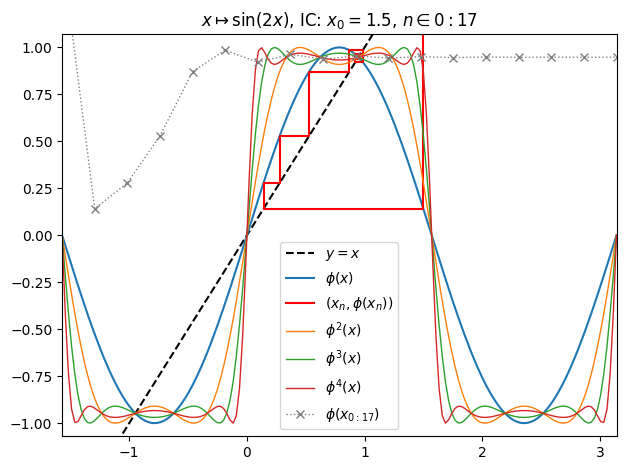

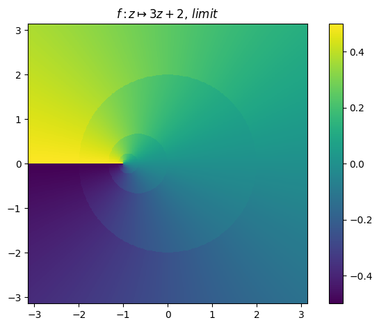
Orbit example (17):

juliafill("3z+2",∂=[-pi,pi],n=500) |> fatou |> plot